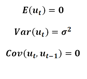
Random Walk Serial Correlation

Both Peak Oxygen Uptake peak VO2, from cardiopulmonary exercise testing CPET and the distance walked during a Six-Minute Walk Test 6 MWD are used for.

Linear regression is the most

widely used of all statistical techniques:

it is the study of linear i.e., straight-line relationships

between variables, usually

under an assumption of normally distributed errors.

The first thing you ought to

know about linear regression is how

the strange term regression came to be applied to

the subject of linear statistical models. This type of predictive

model was first studied in depth by a 19th-Century scientist,

Sir Francis Galton. Galton was a self-taught naturalist,

anthropologist,

astronomer, and statistician--and a real-life Indiana Jones

character. He was famous for his explorations, and he wrote a

best-selling book on how to survive in the wilderness entitled

Shifts and Contrivances Available in Wild Places. The book is still

in print and still considered a useful resource--you

can find a copy in Perkins Library. Among other handy hints for

staying alive--such as how to treat spear-wounds or extract your

horse from quicksand--it introduced the concept of the sleeping

bag to the Western World.

Galton was a pioneer in the

application of statistical methods

to human measurements, and in studying data on relative heights

of fathers and their sons, he observed the following phenomenon: a

taller-than-average father tends to produce a taller-than-average

son, but the son is likely to be less tall than the father

in terms of his relative position within his own population. Thus, for

example, if the father s height is x standard

deviations from the mean within his own population, then you should

predict that the son s height will be rx r times x standard

deviations from the mean within his own population, where r is

a number less than 1 in magnitude. r is what will

be defined below as the correlation between the height

of the father and the height of the son. The same is true of

virtually any physical measurement than can be performed

on parents and their offspring. This seems at first glance like

evidence of some genetic or sociocultural mechanism for damping

out extreme physical traits, and Galton therefore termed it a

regression toward mediocrity, which in modern

terms is a regression to the mean. But the

phenomenon discovered by Galton is a mathematical inevitability:

unless every son is exactly as tall as his father in a

relative sense i.e., unless the correlation is exactly equal

to 1, the predictions must regress to the mean regardless

of the underlying mechanisms of inheritance or culture.

Regression to the mean is an

inescapable fact of life. Your children

can be expected to be less exceptional for better or worse

than you are. Your score on a final exam in a course can be expected

to be less good or bad than your score on the midterm exam.

A baseball player s batting average in the second half of the

season can be expected to be closer to the mean for all

players than his batting average in the first half of the season. And

so on. The key word here is expected. This does

not mean it s certain that regression to the mean will

occur, but that s the way to bet. More precisely, that s the

way to bet if you wish to minimize squared error.

We have already seen a

suggestion of regression-to-the-mean in

some of the time series forecasting models we have studied already:

plots of forecasts tend to be smoother--i.e., they exhibit

less variability--than the plots of the original data. This

is not true of random walk models, but it is generally true of

smoothing models and other models in which coefficients other

than a constant term are estimated. The intuitive explanation

for the regression effect is simple: the thing we are trying

to predict usually consists of a predictable component signal

and a statistically independent unpredictable component

noise. The best we can hope to do is to predict

the value of the signal, and then let the noise fall where it may.

Hence our forecasts will tend to exhibit less variability than

the actual values, which implies a regression to the mean.

Another way to think of the

regression effect is in terms of sampling

bias. Suppose we select a sample of baseball players whose batting

averages were much higher than the mean or students whose grades

were much higher than the mean in the first half of the year.

Presumably their averages were unusually high in part because

they were good and in part because they were lucky. The fact that

they did so well in the first half of the year

makes it probable that both their ability and their luck

were better than average during that period. In the second half

of the year they may be just as good, but they probably will not

be as lucky. So we should predict that in the second half their

performance will be closer to the mean.

Now, why do we often assume

that relationships beween variables

are linear.

Because linear relationships are the simplest

non-trivial

relationships that can be imagined hence the easiest to work

with, and..

Because the true relationships between our variables

are often at least approximately linear over the range

of values that are of interest to us, and

Even if they re not, we can often transform the

variables

in such a way as to linearize the relationships.

And why do we often assume the

errors of linear models are normally

distributed.

This assumption is often justified by

appeal to the central

limit theorem of statistics, which states that the sum

of a sufficiently large number of independent random

variables--whatever

their individual distributions--approaches a normal distribution.

Much data in business and economics is obtained by aggregation--e.g.,

adding up the effects of all transactions occurring in a month,

quarter, year, or whatever. Insofar as individual transactions

may occur randomly and somewhat independently, we might expect

the variations in the aggregate data to be approximately normal

in distribution.

It is again mathematically convenient: it implies that

the

optimal coefficient estimates for a linear model are those that

minimize the mean squared error which are easily calculated,

and it justifies the use of a host of statistical tests based

on the normal family of distributions. This family includes the

t distribution, the F distribution, and the Chi-square distribution.

Even if the true error process is not normal in

terms of the original units of the data, it may be possible to

transform the data so that your model s prediction errors are

approximately normal.

A variable is, by

definition, a quantity that varies. If

it didn t vary, it would be a constant, not a variable. In fitting

statistical models in which some variables are used to predict

others, what we hope to find is that the different variables do

not vary independently in a statistical sense,

but that they tend to vary together.

In particular, when fitting linear

models, we hope to find

that one variable say, Y is varying as a straight-line

function of another variable say, X. In other words, if all

other possibly-relevant variables could be held fixed, we would

hope to find the graph of Y versus X to be a straight

line apart from the inevitable random errors or noise.

A measure of the absolute

amount of variability in

a variable is naturally its variance, which is defined

as its average squared deviation from its own mean.

Equivalently,

we can measure variability in terms of the standard deviation,

which is defined as the square root of the variance. The standard

deviation has the advantage that it is measured in the same units

as the original variable, rather than squared units.

Our task in predicting Y might

be described as that of explaining

some or all of its variance--i.e., why, or under what

conditions,

does it deviate from its mean. Why is it not constant. That is,

we would like to be able to improve on the naive predictive

model: Ý t CONSTANT, in which the best value for the

constant is presumably the historical mean of Y. More precisely,

we hope to find a model whose prediction errors are smaller,

in a mean square sense, than the deviations of the original variable

from its mean.

In using linear models

for prediction, it turns out very

conveniently that the only statistics of interest at least

for purposes of estimating coefficients are the mean and variance

of each variable and the correlation coefficient

between each pair of variables. The coefficient of correlation

between X and Y is commonly denoted by the letter r.

The correlation coefficient

between two variables is a statistic

that measures the strength of the linear relationship between

them, on a relative i.e., unitless scale of -1 to 1. That is,

it measures the extent to which a linear model can be used to

predict the deviation of one variable from its mean given knowledge

of the other s deviation from its mean at the same point in time.

The correlation coefficient is

most easily computed if we first standardize

each of the variables--i.e., express it in units of standard deviations

from its own mean. The standardized value of X is commonly denoted

by X, and the value of X at period t is defined as:

X t X t -

AVERAGE X /STDEV X

where AVERAGE X and STDEV X

are the sample mean average and

standard deviation of X, in Excel notation. For example, suppose

that AVERAGE X 20 and STDEV X 5. If X t 25, then X t

1, if X t 10, then X t -2, and so on.

Now, the correlation

coefficient is equal to the average product

of the standardized values of the two variables. That is,

if we let X and Y denote the standardized values of X and Y,

we have:

r AVERAGE X Y

X 1 Y 1 X 2 Y 2 X n Y n /n

where n is the sample size.

Thus, for example, if X and Y

are stored in columns on a spreadsheet, you can use the AVERAGE

and STDEV functions to compute their averages and standard deviations,

then you can create two new columns in which the values of X

and Y in each period are computed according to the formula above. Then

create a third new column in which X is multiplied by Y

in every period. The average of the values in the last column

is the correlation between X and Y. Of course, in Excel, you

can just use the CORREL x,y function to calculate a correlation

coefficient.

If the two variables tend to

vary on the same sides of

their respective means at the same time, then the average product

of their deviations and hence the correlation between them will

be positive, since the product of two numbers with the

same sign is positive. Conversely, if they tend to vary on opposite

sides of their respective means at the same time, their correlation

will be negative. If they vary independently with

respect to their means--that is, if one is equally likely to be

above or below its mean regardless of what the other is doing--then

the correlation will be zero.

not only the average product of

the standardized values, but also: the correlation coefficient

is the best coefficient for multiplying the standardized

value of one variable in order to predict the standardized value

of the other. That is, the best linear model in

a minimum-squared-error sense for predicting Y from X turns

out to be:

Ý t rX t

Thus, if X is observed to be 1

standard deviation above its own

mean, then we should predict that Y will be r standard deviations

above its own mean; if X is 2 standard deviations below its own

mean, then we should be predict that Y will be 2r standard deviations

below its own mean, and so on.

In graphical terms, this means

that, on a scatter plot of Y versus

X, the best-fit line for predicting Y from X is the line

that passes through the origin and has slope r. Note: this

fact is not supposed to be obvious, but it is easily proved by

elementary differential calculus of several variables.

If we want to obtain a formula

for predicting Y from X in unstandardized

terms, we just need to substitute the formulas for the standardized

values in the prededing equation, which then becomes:

Ý t -

AVERAGE Y /STDEV Y r X t - AVERAGE X /STDEV X

If we now rearrange this

equation and collect constant terms,

we obtain:

Ý t a bX t

where:

b r STDEV Y /STDEV X

a AVERAGE Y -

b AVERAGE X

Notice that, as we claimed

earlier, the coefficients in the linear

equation for predicting Y from X depend only on the means and

standard deviations of X and Y and on their coefficient of correlation.

By the way, these formulas for a and b are mathematically equivalent

to the formulas for b0 and b, respectively,

given on page 206 of your text. Personally, I find it much easier

to remember the formulas in terms of the means and standard deviations

and the correlation coefficient, and I find it easier to write

the formula for the correlation coefficient in terms of the

standardized

values X and Y than in terms of the original values X and Y,

as given on page 204 of your text.

Perfect positive

correlation r 1 or perfect negative

correlation correlation r -1 is only obtained if one variable

is an exact linear function of the other, without error.

In such a case, one variable is merely a linear transformation

of the other--they aren t really different variables

at all.

In general, therefore, we find

less-than-perfect correlation,

which is to say, we find that r is less than 1 in absolute value.

Therefore our prediction for Y will typically be smaller

in absolute value than our observed value for X. That is, we

will always predict Y to be closer to its own mean, in units of

its own standard deviation, than X was observed to be,

which is Galton s phenomenon of regression to the mean.

So, the technical explanation

of the regression-to-the-mean effect

hinges on two mathematical facts: i the correlation coefficient,

calculated in the manner described above, happens to be the coefficient

that minimizes the squared error in predicting Y from X, and

ii the correlation coefficient is never larger than 1 in absolute

value, and it is only equal to 1 when Y is an exact noiseless

linear function of X.

The term regression has stuck

and has even mutated

from an intransitive verb into a transitive one since Galton s

time. We don t merely say that the predictions for Y regress

to the mean --we now say that we are regressing Y on

X when we estimate a linear equation for predicting Y from

X, and we refer to X as a regressor in this case.

When we have fitted a linear

model, we can compute its mean squared

prediction error and compare this to the variance of the original

variable. As noted above, we hope to find that the MSE is less

than the original variance. The relative amount by which the mean

squared error is less than the variance of the original variable

is referred to as the fraction of the variance that was

explained by the model. For example, if the MSE is 20

less than the original variance, we say we have explained

20 of the variance.

It turns out that in a

simple regression model a linear

model with only one X variable, the fraction

of variance explained is precisely the square of the correlation

coefficient--i.e., the square of r. Hence, the

fraction-of-variance-explained

has come to be known as r-squared.

In a multiple regression model a linear model with

two

or more regressors, there are many correlation coefficients

that must be computed, in addition to all the means and variances.

For example, we must consider the correlation between each

X variable and the Y variable, and also the correlation between

each pair of X variables. In this case, it still

turns

out that the model coefficients and the fraction-of-variance-explained

statistic can be computed entirely from knowledge of the means,

standard deviations, and correlation coefficients among the

variables--but

the computations are no longer easy. We will leave the details

to the computer.

• Random Walks in Stock- Market Prices FOR MANY YEARSeconomists, statisticians, and teachers of finance have been inter-ested in developing and testing models of.
• Linear regression analysis is the most widely used of all statistical techniques: it is the study of linear, additive relationships between variables.
• 2SLS: an abbreviation for two stage least squares, an instrumental variables estimation technique. Contexts: econometrics; estimation 3SLS: A kind of simultaneous.

1965-1974 Random Walks in Stock Market Prices Eugene F. Fama For many years economists, statisticians, and teachers of finance have been interested in.

Statistical Testing of Random Number Generators Juan Soto National Institute of Standards Technology. 100 Bureau Drive, Stop 8930. Gaithersburg, MD 20899-8930.

Nonstationary expected returns: Implications for tests of market efficiency and serial correlation in returns.

Real Business Cycles RBC theory views cycles as arising in frictionless perfectly competitive economies with generally complete markets subject to real shocks.